Exploratory Data Analysis

BIOSTAT 620: Introduction to Health Data Science

Dylan Cable

Exploratory Data Analysis

Main topic for today

Acknowledgment

This lecture includes some slides originally developed by Meredith Franklin. They have been modified by George G. Vega Yon, Kelly Street, and Dylan Cable.

Exploratory Data Analysis

Exploratory data analysis is the process of becoming familiar with a dataset
It should be the first step in your analysis pipeline
It involves:
- checking data (import issues, outliers, missing values, data errors)
- cleaning data
- summary statistics of key variables (univariate and bivariate)
- basic plots and graphs

Exploratory Data Analysis

Since our eyes and brains are not wired to detect patterns in large data tables filled with text and numbers, communication about data […] rarely comes in the form of raw data or code output. Instead, data and data-driven results are usually either summarized (e.g., using an average/mean) and presented in small summary tables or they are presented visually in the form of graphs, in which shape, distance, color, and size can be used to represent the magnitudes of (and relationships between) the values within our data.

Viridical Data Science, Yu and Barter

Key Questions

What question(s) am I trying to answer?
What question(s) could this dataset answer?

The Tidyverse Model

Loosely, EDA encompasses the Import -> Tidy -> Transform -> Visualize steps. Basically it is everything before we do modeling, prediction or inference.

EDA may involve some statistical summaries, but it does not include formal statistical analysis.

EDA Checklist

The goal of EDA is to better understand your data. Let’s use the checklist:

Read in the data
Check the size of the data
Examine the variables and their types
Look at the top and bottom of the data
Visualize the distributions of key variables
Check your expectations
Validate with an external source
Formulate a (simple) question
Try the easy solution first
Challenge your solution

(adapted from Exploratory Data Analysis with R by Roger D. Peng)

Case study

We are going to use a dataset created from the National Center for Environmental Information (https://www.ncei.noaa.gov/). The data are 2019 hourly measurements from weather stations across the continental U.S.

Formulate a Question

It is a good idea to first have a question such as:

Which weather stations reported the hottest and coldest daily temperatures?
What day of the month was on average the hottest?
Is there correlation between temperature and humidity in my dataset?

Read in the Data

There are several ways to read in data (some depend on the type of data you have):

read.table or read.csv in base R for delimited files
readRDS if you have a .rds dataset (this is a handy, compressed way of saving R objects)
read_csv, read_csv2, read_delim, read_fwf from library(readr) that is part of the tidyverse
readxl() from library(readxl) for .xls and .xlsx files
read_sas, read_spss, read_stata from library(haven)
fread from library(data.table) for efficiently importing large datasets that are regular delimited files

Read in the Data

There are plenty of ways to do these tasks, but we will focus on base R.

Since our data is stored as a (gzipped) CSV file, we could load it into R with read.csv, but we will use the more flexible read.table. I have it stored locally, but we will see how to load it straight from GitHub in the lab.

met <- read.table('../data/met/met_all.gz',
                  header = TRUE, sep = ',')

We specify that the first line contains column names by setting header = TRUE and we indicate that commas are used to separate the different values (rather than tabs, spaces, etc.) by setting sep = ','.

Working with `data.frame`s

This gave as a data.frame object, which is a standard R format for cleaned, rectangular data. Each row represents an observation and each column represents a variable.

As we have seen, you can access particular parts of the data.frame by subsetting with the square brackets, [,]. For example, you can pull out the 2nd, 3rd, and 4th elements of the 1st column of our met dataset with met[2:4, 1].

You can also pull out specific columns by name, using the $ operator. Since the first column is called USAFID, we could access the same subset as above with met$USAFID[2:4] (notice that there is no comma here, because we have already subset down to a single variable).

To see the list of names for the dataset, you can use names(met) or colnames(met). To see the top few rows of the dataset, use head(met).

Check the data

We should check the dimensions of the data set. This can be done several ways:

dim(met)

[1] 2377343      30

nrow(met)

[1] 2377343

ncol(met)

[1] 30

Check the data

We see that there are 2,377,343 records of hourly temperature in August 2019 from all of the weather stations in the US. The data set has 30 variables.
We should also check the top and bottom of the dataset to check for any irregularities. Use head(met) and tail(met) for this.
Next we can take a deeper dive into the contents of the data with str()

Check variables

str(met)

'data.frame':   2377343 obs. of  30 variables:
 $ USAFID           : int  690150 690150 690150 690150 690150 690150 690150 690150 690150 690150 ...
 $ WBAN             : int  93121 93121 93121 93121 93121 93121 93121 93121 93121 93121 ...
 $ year             : int  2019 2019 2019 2019 2019 2019 2019 2019 2019 2019 ...
 $ month            : int  8 8 8 8 8 8 8 8 8 8 ...
 $ day              : int  1 1 1 1 1 1 1 1 1 1 ...
 $ hour             : int  0 1 2 3 4 5 6 7 8 9 ...
 $ min              : int  56 56 56 56 56 56 56 56 56 56 ...
 $ lat              : num  34.3 34.3 34.3 34.3 34.3 34.3 34.3 34.3 34.3 34.3 ...
 $ lon              : num  -116 -116 -116 -116 -116 ...
 $ elev             : int  696 696 696 696 696 696 696 696 696 696 ...
 $ wind.dir         : int  220 230 230 210 120 NA 320 10 320 350 ...
 $ wind.dir.qc      : chr  "5" "5" "5" "5" ...
 $ wind.type.code   : chr  "N" "N" "N" "N" ...
 $ wind.sp          : num  5.7 8.2 6.7 5.1 2.1 0 1.5 2.1 2.6 1.5 ...
 $ wind.sp.qc       : chr  "5" "5" "5" "5" ...
 $ ceiling.ht       : int  22000 22000 22000 22000 22000 22000 22000 22000 22000 22000 ...
 $ ceiling.ht.qc    : int  5 5 5 5 5 5 5 5 5 5 ...
 $ ceiling.ht.method: chr  "9" "9" "9" "9" ...
 $ sky.cond         : chr  "N" "N" "N" "N" ...
 $ vis.dist         : int  16093 16093 16093 16093 16093 16093 16093 16093 16093 16093 ...
 $ vis.dist.qc      : chr  "5" "5" "5" "5" ...
 $ vis.var          : chr  "N" "N" "N" "N" ...
 $ vis.var.qc       : chr  "5" "5" "5" "5" ...
 $ temp             : num  37.2 35.6 34.4 33.3 32.8 31.1 29.4 28.9 27.2 26.7 ...
 $ temp.qc          : chr  "5" "5" "5" "5" ...
 $ dew.point        : num  10.6 10.6 7.2 5 5 5.6 6.1 6.7 7.8 7.8 ...
 $ dew.point.qc     : chr  "5" "5" "5" "5" ...
 $ atm.press        : num  1010 1010 1011 1012 1013 ...
 $ atm.press.qc     : int  5 5 5 5 5 5 5 5 5 5 ...
 $ rh               : num  19.9 21.8 18.5 16.9 17.4 ...

Check variables

First, we see that str() gives us the class of the data, which in this case is a data.frame, as well as the dimensions of the data
We also see the variable names and their type (integer, numeric, character, etc.)
We can identify major problems with the data at this stage (e.g. a variable that has all missing values)

Check variables

We can get summary statistics on our data.frame using summary().

summary(met[,8:13])

      lat             lon               elev           wind.dir     
 Min.   :24.55   Min.   :-124.29   Min.   : -13.0   Min.   :  3     
 1st Qu.:33.97   1st Qu.: -98.02   1st Qu.: 101.0   1st Qu.:120     
 Median :38.35   Median : -91.71   Median : 252.0   Median :180     
 Mean   :37.94   Mean   : -92.15   Mean   : 415.8   Mean   :185     
 3rd Qu.:41.94   3rd Qu.: -82.99   3rd Qu.: 400.0   3rd Qu.:260     
 Max.   :48.94   Max.   : -68.31   Max.   :9999.0   Max.   :360     
                                                    NA's   :785290  
 wind.dir.qc        wind.type.code    
 Length:2377343     Length:2377343    
 Class :character   Class :character  
 Mode  :character   Mode  :character

Check variables more closely

We know that we are supposed to have hourly measurements of weather data for the month of August 2019 for the entire US. We should check that we have all of these components. Let’s check:

the year
the month
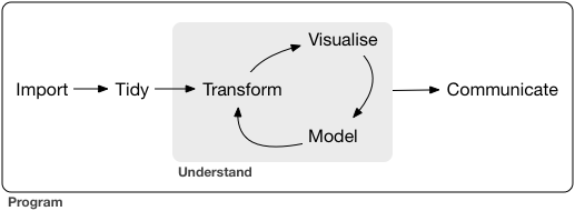
the hours
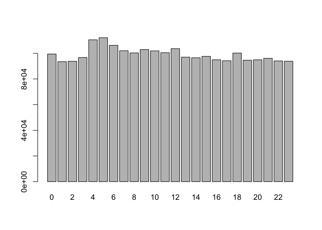
the range of locations (latitude and longitude)

Check variables more closely

We can generate tables and/or barplots for integer variables:

table(met$hour)


     0      1      2      3      4      5      6      7      8      9     10 
 99434  93482  93770  96703 110504 112128 106235 101985 100310 102915 101880 
    11     12     13     14     15     16     17     18     19     20     21 
100470 103605  97004  96507  97635  94942  94184 100179  94604  94928  96070 
    22     23 
 94046  93823

table(met$month)


      8 
2377343

Check variables more closely

We can generate tables and/or barplots for integer variables:

barplot(table(met$hour))

Check variables more closely

For numeric variables we should do a summary to see the quantiles, min, max, and mean.

table(met$year)


   2019 
2377343

summary(met$lat)

   Min. 1st Qu.  Median    Mean 3rd Qu.    Max. 
  24.55   33.97   38.35   37.94   41.94   48.94

summary(met$lon)

   Min. 1st Qu.  Median    Mean 3rd Qu.    Max. 
-124.29  -98.02  -91.71  -92.15  -82.99  -68.31

Check variables more closely

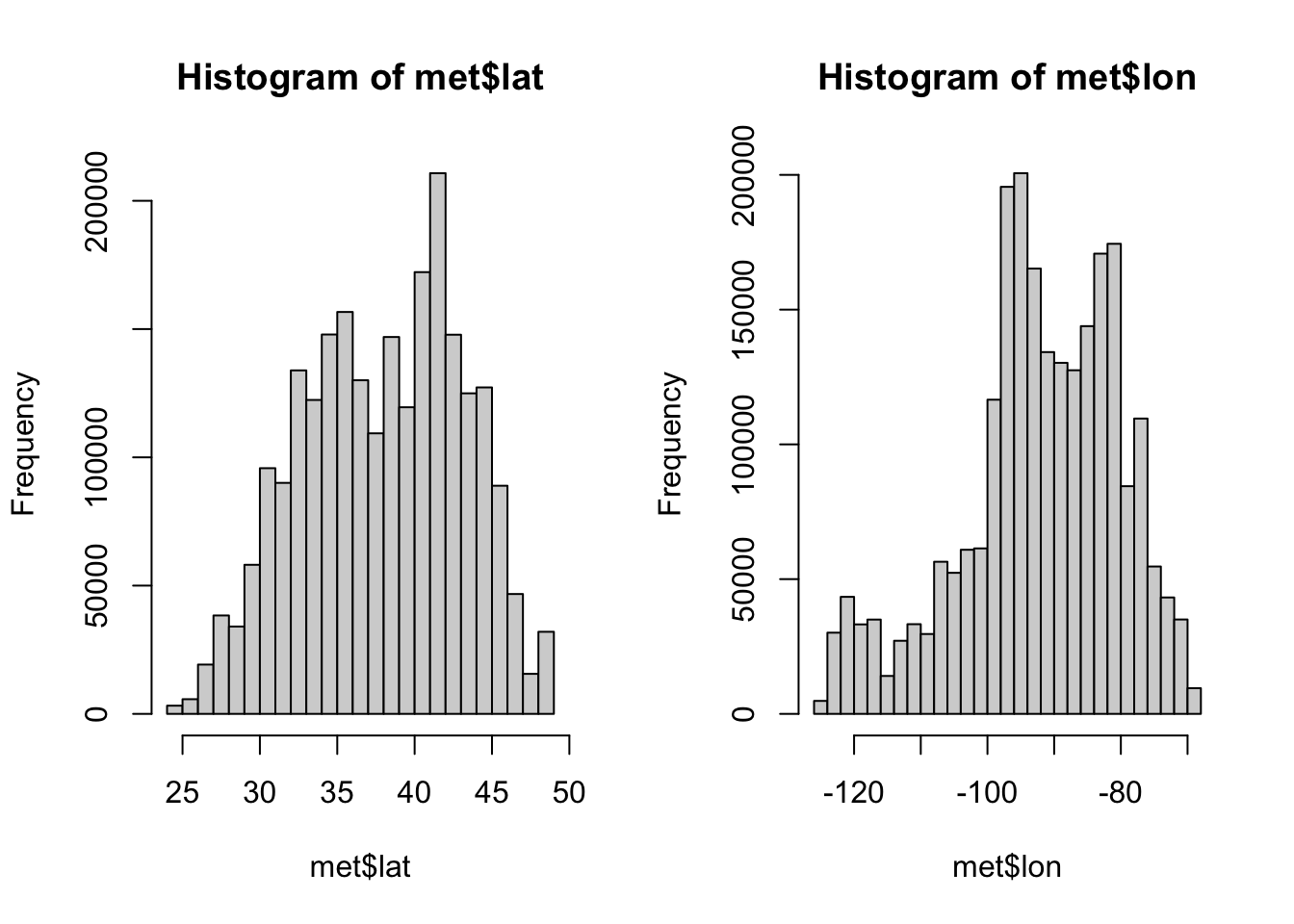
We can visualize these distributions with a histogram.

layout(matrix(1:2, nrow=1))
hist(met$lat)
hist(met$lon)

layout(1)

Check variables more closely

If we return to our initial question, what weather stations reported the hottest and coldest temperatures, we should take a closer look at our key variable, temperature (temp)

summary(met$temp)

   Min. 1st Qu.  Median    Mean 3rd Qu.    Max.    NA's 
 -40.00   19.60   23.50   23.59   27.80   56.00   60089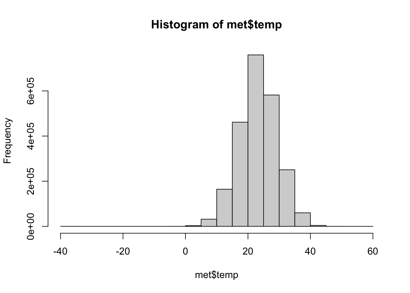

hist(met$temp)

It looks like the temperatures are in Celsius. A temperature of -40 in August is really cold, we should see if this is an implausible value.

Check variables more closely

It also looks like there is a lot of missing data, encoded by NA values. Let’s check the proportion of missingness by tallying up whether or not every temperature reading is an NA. This will give us a vector of TRUE/FALSE values and then we can take the mean (average), because R automatically interprets TRUE as 1 and FALSE as 0 for mathematical functions.

mean(is.na(met$temp))

[1] 0.0252757

2.5% of the data are missing, which is not a huge amount.

Check variables more closely

In our data.frame we can easily subset the data and select certain columns. Here, we select all observations with a temperature of -40C and a specific subset of the variables:

met_ss <- met[met$temp == -40.00, c('hour','lat','lon','elev','wind.sp')]

dim(met_ss)

[1] 60125     5

summary(met_ss)

      hour            lat             lon              elev      
 Min.   : 0.00   Min.   :29.12   Min.   :-89.55   Min.   :36     
 1st Qu.: 2.75   1st Qu.:29.12   1st Qu.:-89.55   1st Qu.:36     
 Median : 5.50   Median :29.12   Median :-89.55   Median :36     
 Mean   : 5.50   Mean   :29.12   Mean   :-89.55   Mean   :36     
 3rd Qu.: 8.25   3rd Qu.:29.12   3rd Qu.:-89.55   3rd Qu.:36     
 Max.   :11.00   Max.   :29.12   Max.   :-89.55   Max.   :36     
 NA's   :60089   NA's   :60089   NA's   :60089    NA's   :60089  
    wind.sp     
 Min.   : NA    
 1st Qu.: NA    
 Median : NA    
 Mean   :NaN    
 3rd Qu.: NA    
 Max.   : NA    
 NA's   :60125

Check variables more closely

In dplyr we can do the same thing using filter and select

library(dplyr)
met_ss <- filter(met, temp == -40.00) |> 
  select(USAFID, day, hour, lat, lon, elev, wind.sp)

dim(met_ss)

[1] 36  7

summary(met_ss)

     USAFID            day         hour            lat             lon        
 Min.   :720717   Min.   :1   Min.   : 0.00   Min.   :29.12   Min.   :-89.55  
 1st Qu.:720717   1st Qu.:1   1st Qu.: 2.75   1st Qu.:29.12   1st Qu.:-89.55  
 Median :720717   Median :1   Median : 5.50   Median :29.12   Median :-89.55  
 Mean   :720717   Mean   :1   Mean   : 5.50   Mean   :29.12   Mean   :-89.55  
 3rd Qu.:720717   3rd Qu.:1   3rd Qu.: 8.25   3rd Qu.:29.12   3rd Qu.:-89.55  
 Max.   :720717   Max.   :1   Max.   :11.00   Max.   :29.12   Max.   :-89.55  
                                                                              
      elev       wind.sp   
 Min.   :36   Min.   : NA  
 1st Qu.:36   1st Qu.: NA  
 Median :36   Median : NA  
 Mean   :36   Mean   :NaN  
 3rd Qu.:36   3rd Qu.: NA  
 Max.   :36   Max.   : NA  
              NA's   :36

Validate against an external source

We should check outside sources to make sure that our data makes sense. For example the observation with -40C is suspicious, so we should look up the location of the weather station.

Go to Google maps and enter the coordinates for the site with -40C (29.12, -89.55)

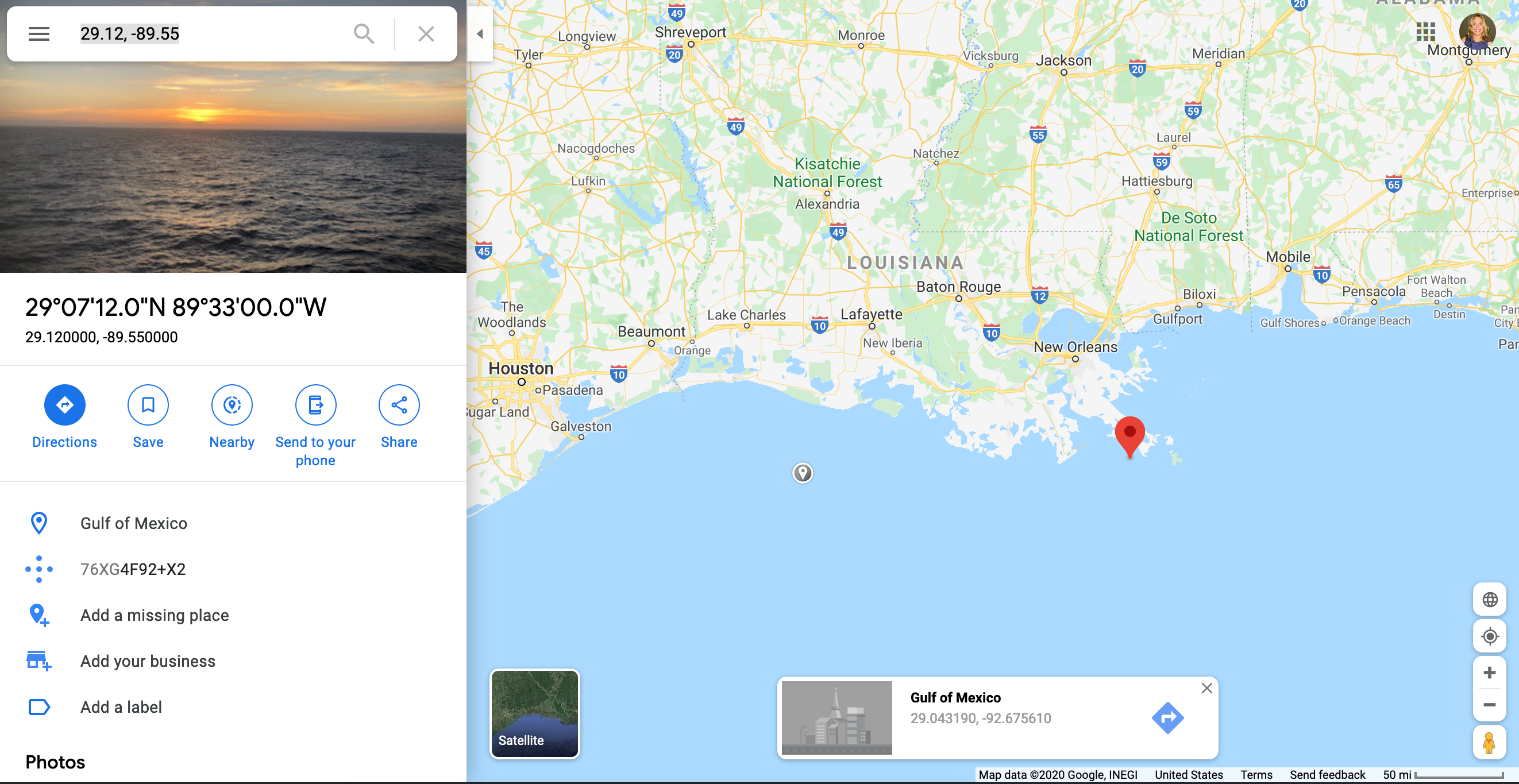
It doesn’t make much sense to have a -40C reading in the Gulf of Mexico off the coast of Louisiana!

Data cleaning

If we return to our initial question (“Which weather stations reported the hottest and coldest daily temperatures?”), we need to generate a list of weather stations that are ordered from highest to lowest. We can then examine the top and bottom of this new dataset.

First let us remove the aberrant observations and then we’ll sort by temperature.

met <- met[met$temp > -40, ]

Notice that we do not create a new object, we just overwrite the met object. Once you’re sure that you want to remove certain observations, this is a good way to avoid confusion (otherwise, it is easy to end up with multiple subsets of the data in your R environment with similar names like met, met_ss, met_ss2, met_final, met_FINAL, met_FINAL_REAL, etc.)

Data cleaning

We will also remove any observations with missing temperature values (NA).

The is.na() function tells you whether or not a particular value is missing and the ! operator takes the opposite of a TRUE/FALSE value, so in combination, they tell you which observations are not missing.

met <- met[!is.na(met$temp), ]

Sorting

Now, we can use the order() function to sort our dataset.

met <- met[order(met$temp), ]

Again, we just replace the met object with this updated version, since we aren’t actually losing any data, just changing the order.

Highest and Lowest

head(met)[,c(1,8:10,24)]

        USAFID    lat    lon elev  temp
1203053 722817 38.767 -104.3 1838 -17.2
1203055 722817 38.767 -104.3 1838 -17.2
1203128 722817 38.767 -104.3 1838 -17.2
1203129 722817 38.767 -104.3 1838 -17.2
1203222 722817 38.767 -104.3 1838 -17.2
1203225 722817 38.767 -104.3 1838 -17.2

tail(met)[,c(1,8:10,24)]

      USAFID    lat      lon elev temp
42783 720267 38.955 -121.081  467 52.0
724   690150 34.300 -116.166  696 52.8
749   690150 34.296 -116.162  625 52.8
748   690150 34.300 -116.166  696 53.9
701   690150 34.300 -116.166  696 54.4
42403 720267 38.955 -121.081  467 56.0

Summary statistics

The maximum hourly temperature is 56C at site 720267, and the minimum hourly temperature is -17.2C at site 722817.

Summary statistics

We need to transform our data to answer our initial question. Let’s find the daily mean, max, and min temperatures for each weather station in our data.frame. We can do this with the summarize function from the dplyr package. This package is part of the tidyverse, so the syntax is a bit different from what we’ve seen before.

library(dplyr)
met_daily <- summarize(met,
                       temp = mean(temp),
                       lat = mean(lat),
                       lon = mean(lon),
                       elev = mean(elev),
                       .by = c(USAFID, day))

What we’ve done here is told R to summarize the met dataset by the variables USAFID and day, splitting the data into subsets based on those two indexing variables. For each subset (representing a specific station of a specific day), we want the daily average temperature, as well as latitude, longitude, and elevation (though hopefully those don’t change too much over the course of a day!)

Summary statistics

Before we continue, check the relative sizes of the met and met_daily objects. Which one is bigger?

Summary statistics

Now we will order our new dataset by the average daily temperature, just as we ordered the old one by observed temperature.

met_daily <- met_daily[order(met_daily$temp), ]

head(met_daily)

    USAFID day       temp    lat    lon elev
2   722817   3 -17.200000 38.767 -104.3 1838
1   722817   1 -17.133333 38.767 -104.3 1838
3   722817   6 -17.066667 38.767 -104.3 1838
164 726130  11   4.278261 44.270  -71.3 1909
166 726130  31   4.304348 44.270  -71.3 1909
163 726130  10   4.583333 44.270  -71.3 1909

tail(met_daily)

      USAFID day     temp      lat       lon     elev
48708 722749   5 40.85714 33.26900 -111.8120 379.0000
48695 723805   5 40.97500 34.76800 -114.6180 279.0000
48721 720339  14 41.00000 32.14600 -111.1710 737.0000
48710 723805   4 41.18333 34.76800 -114.6180 279.0000
48688 722787   5 41.35714 33.52700 -112.2950 325.0000
48438 690150  31 41.71667 34.29967 -116.1657 690.0833

Summary statistics

The maximum daily average temperature is 41.7166667 C at site 690150 and the minimum daily average temperature is -17.2C at site 722817.

Summary statistics

The code below is similar to our previous example, but doesn’t include the latitude, longitude, and elevation. How would you alter this code to find the daily median, max, or min temperatures for each station?

summarize(met,
          temp = mean(temp),
          .by = c(USAFID, day))

(try it yourself)

Exploratory graphs

With exploratory graphs we aim to:

debug any issues remaining in the data
understand properties of the data
look for patterns in the data
inform modeling strategies

Exploratory graphs do not need to be perfect, we will look at presentation ready plots next week.

Exploratory graphs

Examples of exploratory graphs include:

histograms
boxplots
scatterplots
simple maps

Exploratory Graphs

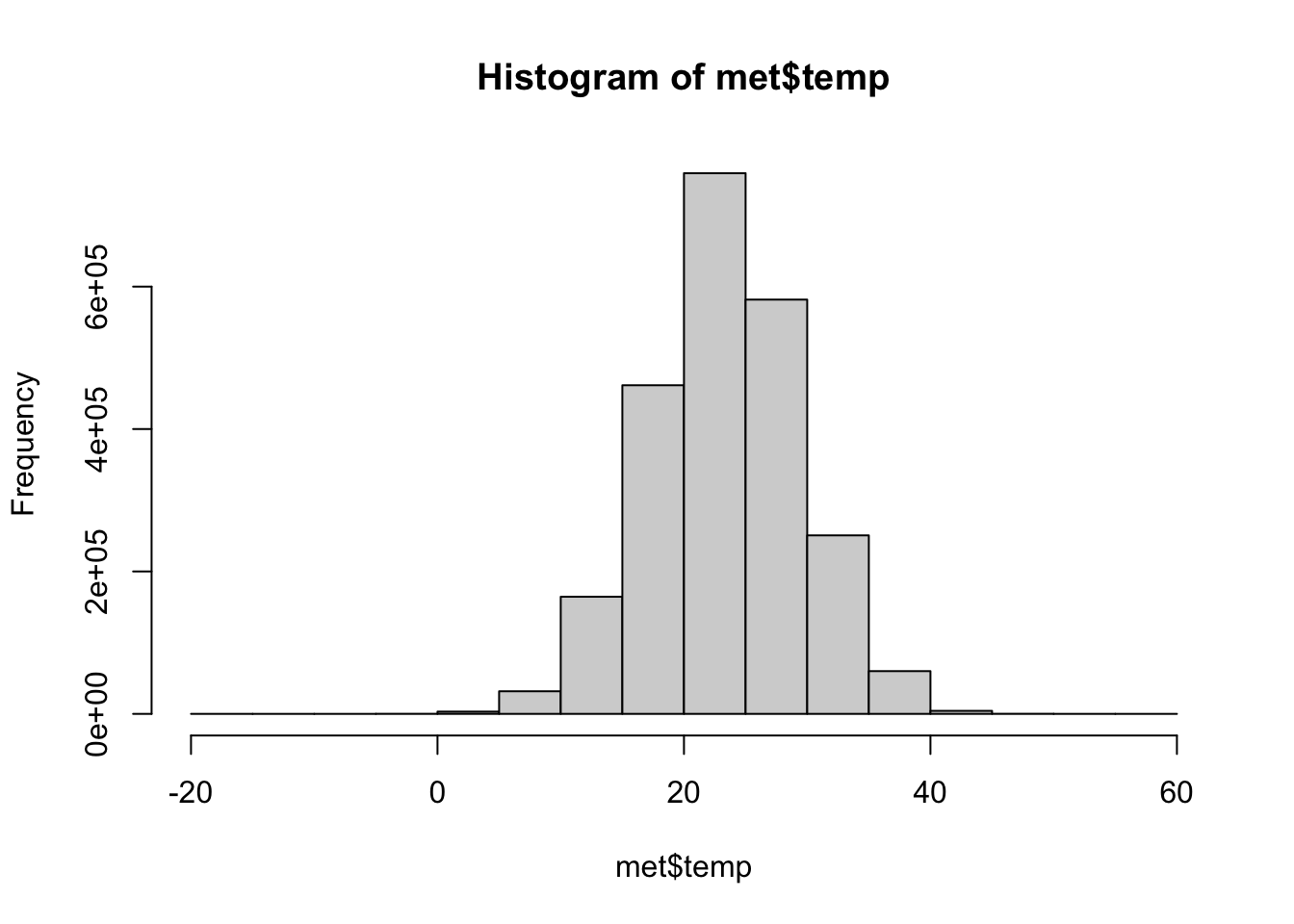
Focusing on the variable of interest, temperature, let’s look at the distribution (after removing -40C)

hist(met$temp)

Exploratory Graphs

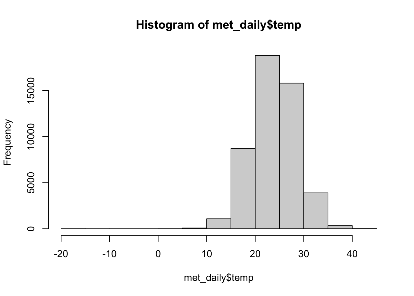
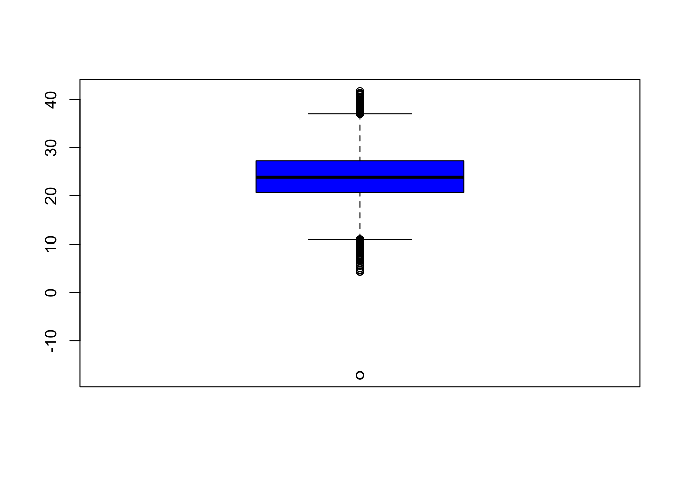
Let’s look at the daily data

hist(met_daily$temp)

Exploratory Graphs

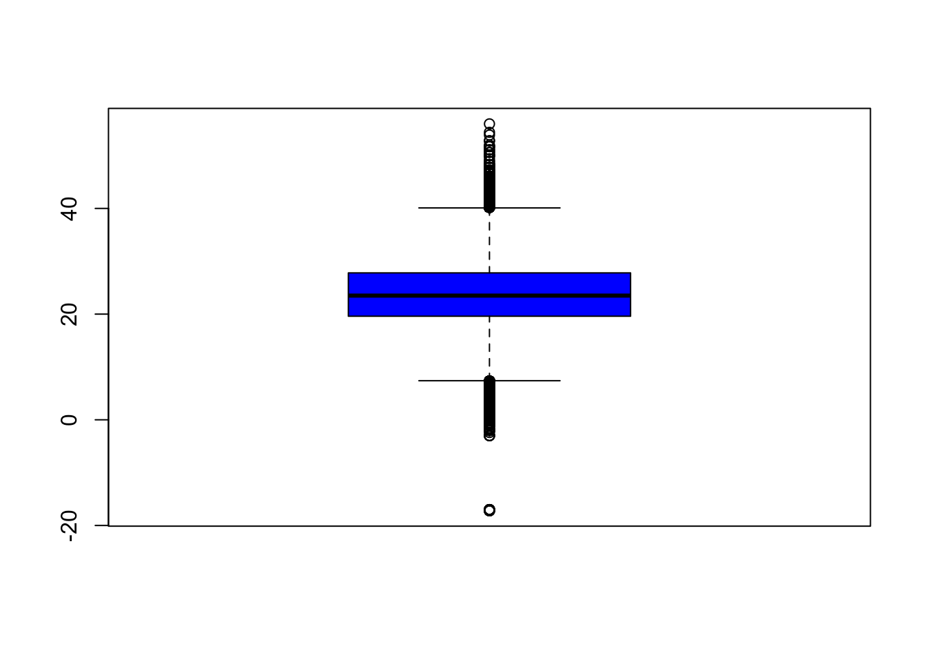
A boxplot gives us an idea of the quantiles of the distribution and any outliers

boxplot(met$temp, col = "blue")

Exploratory Graphs

Let’s look at the daily data

boxplot(met_daily$temp, col = "blue")

Exploratory Graphs

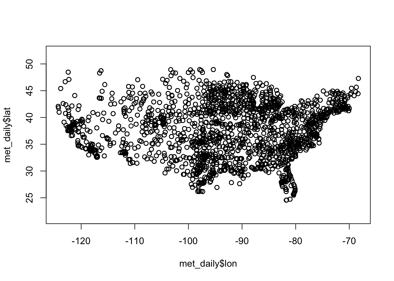
We know that these data come from US weather stations, so we might have some idea what to expect just from plotting the latitude and longitude (note that we fix the aspect ratio at 1:1 with asp = 1; this prevents the plot from stretching or shrinking to fit the available plotting area):

plot(met_daily$lon, met_daily$lat, asp=1)

Exploratory Graphs

A map will show us where the weather stations are located. First let’s get the unique latitudes and longitudes and see how many meteorological sites there are

met_stations <- (unique(met[,c("lat","lon")]))  
dim(met_stations)

[1] 2827    2

Exploratory Graphs

A map will show us where the weather stations are located. First let’s get the unique latitudes and longitudes and see how many meteorological sites there are.

library(leaflet)
leaflet(met_stations) |> 
  addProviderTiles('CartoDB.Positron') |> 
  addCircles(lat = ~lat, lng = ~lon,
             opacity = 1, fillOpacity = 1, radius = 400)

Exploratory Graphs

Let’s map the locations of the max and min daily temperatures.

min <- met_daily[1, ]               # First observation
max <- met_daily[nrow(met_daily), ] # Last observation

leaflet() |> 
  addProviderTiles('CartoDB.Positron') |> 
  addCircles(
    data = min,
    lat = ~lat, lng = ~lon, popup = "Min temp.",
    opacity = 1, fillOpacity = 1, radius = 400, color = "blue"
    ) |>
  addCircles(
    data = max,
    lat = ~lat, lng = ~lon, popup = "Max temp.",
    opacity=1, fillOpacity=1, radius = 400, color = "red"
    )

(next slide)

Exploratory Graphs

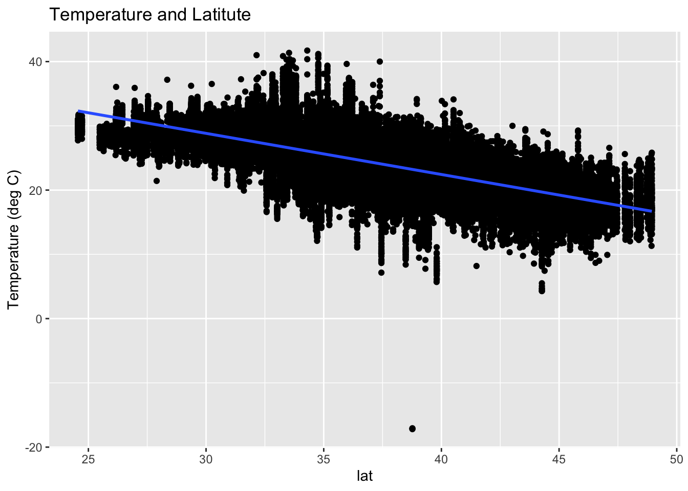
Scatterplots help us look at pairwise relationships. Let’s see if there is any trend in temperature with latitude

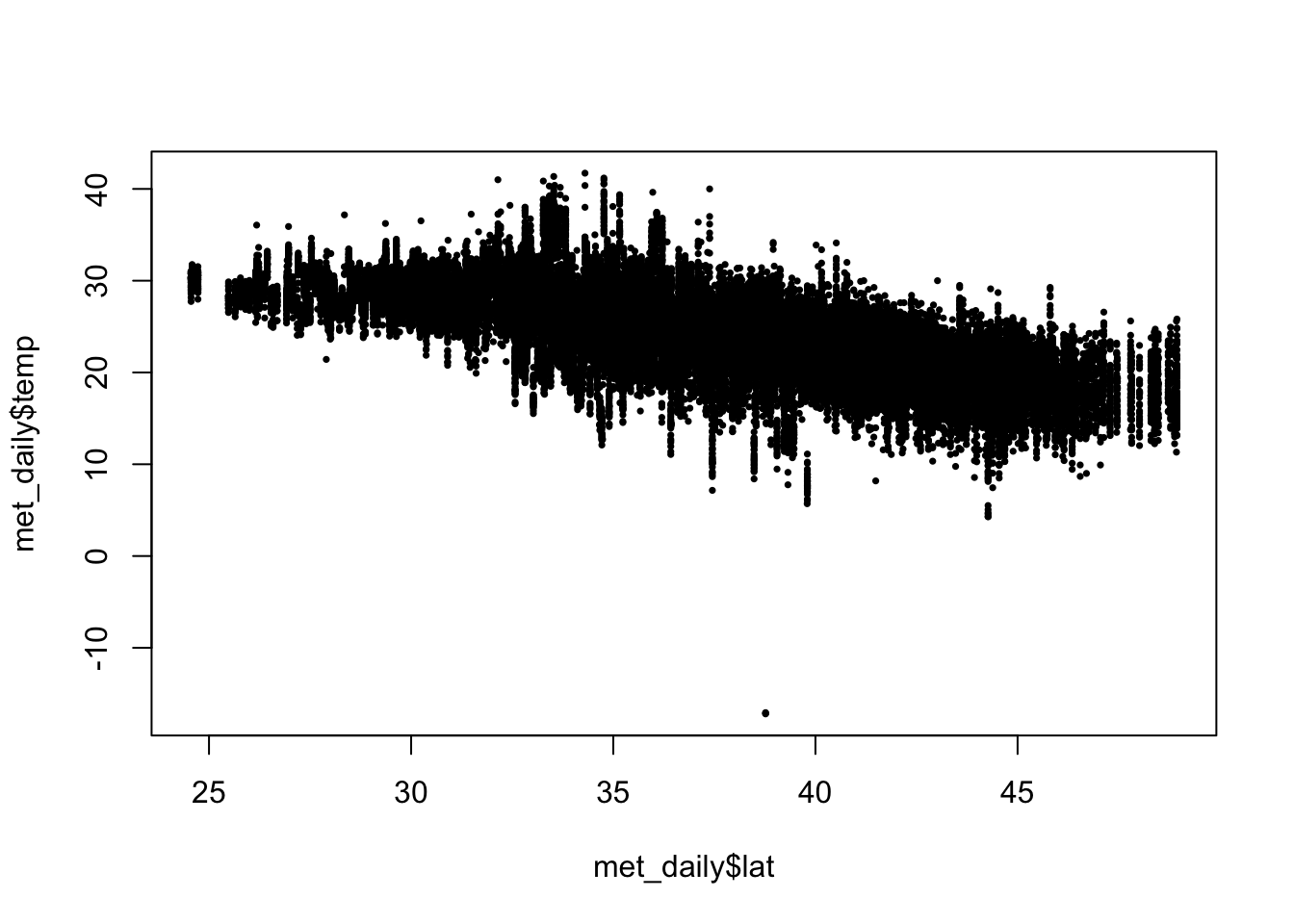
plot(met_daily$lat, met_daily$temp, pch=16, cex=0.5)

There is a clear decrease in temperatures as you increase in latitude (i.e as you go north).

Exploratory Graphs

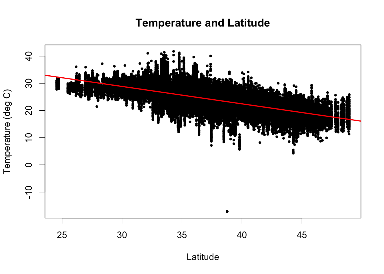
We can add a simple linear regression line to this plot using lm() and abline(). We can also add a title and change the axis labels.

mod <- lm(temp ~ lat, data = met_daily)
plot(met_daily$lat, met_daily$temp, pch=19, cex=0.5, 
  main = "Temperature and Latitude", 
  xlab = "Latitude", ylab = "Temperature (deg C)")
abline(mod, lwd=2, col="red")

(next slide)

Using ggplot2 (next class)

library(ggplot2)
ggplot(data = met_daily, mapping = aes(x = lat, y = temp)) +
  geom_point() + geom_smooth(method = "lm", se = FALSE) +
  labs(title = "Temperature and Latitute", xlab  = "Latitute", y = "Temperature (deg C)")

Summary

In EDA we:

have an initial question that we aim to answer
import, check, clean the data
perform any data transformations to answer the initial question
make some basic graphs to examine the data and visualize the initial question

Next topic (starting today): Tidyverse

Tidyverse

library(tidyverse)

The tidyverse is not a package but a group of packages developed to work with each other.
The tidyverse makes data analysis simpler and code easier to read by sacrificing some flexibility.
One way code is simplified by ensuring all functions take and return tidy data.

Tidy data

Stored in a data frame.
Each observation is exactly one row.
Variables are stored in columns.
Not all data can be represented this way, but a very large subset of data analysis challenges are based on tidy data.
Assuming data is tidy simplifies coding and frees up our minds for statistical thinking.

Tidy data

This is an example of a tidy dataset:

      country year fertility
1     Germany 1960      2.41
2 South Korea 1960      6.16
3     Germany 1961      2.44
4 South Korea 1961      5.99
5     Germany 1962      2.47
6 South Korea 1962      5.79

Tidy data

Originally, the data was in the following format:

      country 1960 1961 1962 1963 1964 1965 1966 1967 1968 1969 1970
1     Germany 2.41 2.44 2.47 2.49 2.49 2.48 2.44 2.37 2.28 2.17 2.04
2 South Korea 6.16 5.99 5.79 5.57 5.36 5.16 4.99 4.85 4.73 4.62 4.53

This is not tidy.

Tidyverse packages

tibble - improves data frame class.
readr - import data.
dplyr - used to modify data frames.
ggplot2 - simplifies plotting.
tidyr - helps convert data into tidy format.
stringr - string processing.
forcats - utilities for categorical data.
purrr - tidy version of apply functions.

dplyr

In this lecture we focus mainly on dplyr.
In particular the following functions:
- mutate
- select
- across
- filter
- group_by
- summarize

Adding a column with `mutate`

murders <- mutate(murders, rate = total/population*100000)

Notice that here we used total and population inside the function, which are objects that are not defined in our workspace.
This is known as non-standard evaluation where the context is used to know what variable names means.
Tidyverse extensively uses non-standard evaluation.
This can create confusion but it certainly simplifies code.

Subsetting with `filter`

filter(murders, rate <= 0.71)

          state abb        region population total      rate
1        Hawaii  HI          West    1360301     7 0.5145920
2          Iowa  IA North Central    3046355    21 0.6893484
3 New Hampshire  NH     Northeast    1316470     5 0.3798036
4  North Dakota  ND North Central     672591     4 0.5947151
5       Vermont  VT     Northeast     625741     2 0.3196211

Selecting columns with `select`

new_table <- select(murders, state, region, rate)
filter(new_table, rate <= 0.71)

          state        region      rate
1        Hawaii          West 0.5145920
2          Iowa North Central 0.6893484
3 New Hampshire     Northeast 0.3798036
4  North Dakota North Central 0.5947151
5       Vermont     Northeast 0.3196211

Transforming variables

The function mutate can also be used to transform variables.
For example, the following code takes the log transformation of the population variable:

mutate(murders, population = log10(population))

Transforming variables

Often, we need to apply the same transformation to several variables.
The function across facilitates the operation.
For example if want to log transform both population and total murders we can use:

mutate(murders, across(c(population, total), log10))

Transforming variables

The helper functions come in handy when using across.
An example is if we want to apply the same transformation to all numeric variables:

mutate(murders, across(where(is.numeric), log10))

or all character variables:

mutate(murders, across(where(is.character), tolower))

There are several other useful helper functions.

The pipe: `|>` or `%>%`

We use the pipe to chain a series of operations.
For example if we want to select columns and then filter rows we chain like this:

\[ \mbox{original data } \rightarrow \mbox{ select } \rightarrow \mbox{ filter } \]

The pipe: `|>` or `%>%`

The code looks like this:

murders |> select(state, region, rate) |> filter(rate <= 0.71)

          state        region      rate
1        Hawaii          West 0.5145920
2          Iowa North Central 0.6893484
3 New Hampshire     Northeast 0.3798036
4  North Dakota North Central 0.5947151
5       Vermont     Northeast 0.3196211

The object on the left of the pipe is used as the first argument for the function on the right.
The second argument becomes the first, the third the second, and so on…

The pipe: `|>` or `%>%`

Here is a simple example:

16 |> sqrt() |> log(base = 2)

[1] 2

Summarizing data

We use the dplyr summarize function, not to be confused with summary from R base.
Here is an example of how it works:

murders |> summarize(avg = mean(rate))

       avg
1 2.779125

Let’s compute murder rate for the US. Is the above it?

Summarizing data

No, the rate is NOT the average of rates.
It is the total murders divided by total population:

murders |> summarize(rate = sum(total)/sum(population)*100000)

      rate
1 3.034555

Multiple summaries

Suppose we want the median, minimum and max population size:

murders |> summarize(median = median(population), min = min(population), max = max(population))

   median    min      max
1 4339367 563626 37253956

Why don’t we use quantiles?

murders |> summarize(quantiles = quantile(population, c(0.5, 0, 1)))

  quantiles
1   4339367
2    563626
3  37253956

Multiple summaries

Warning

Using a function that returns more than one number within summarize will soon be deprecated.

For multiple summaries we use reframe:

murders |> reframe(quantiles = quantile(population, c(0.5, 0, 1)))

  quantiles
1   4339367
2    563626
3  37253956

Multiple summaries

However, if we want a column per summary, as when we called min, median, and max separately, we have to define a function that returns a data frame like this:

median_min_max <- function(x){
  qs <- quantile(x, c(0.5, 0, 1))
  data.frame(median = qs[1], min = qs[2], max = qs[3])
}

Then we can call summarize:

murders |> summarize(median_min_max(population))

   median    min      max
1 4339367 563626 37253956

Group then summarize

Let’s compute murder rate by region.
Take a close look at this output?

murders |> group_by(region) |> head(4)

# A tibble: 4 × 6
# Groups:   region [2]
  state    abb   region population total  rate
  <chr>    <chr> <fct>       <dbl> <dbl> <dbl>
1 Alabama  AL    South     4779736   135  2.82
2 Alaska   AK    West       710231    19  2.68
3 Arizona  AZ    West      6392017   232  3.63
4 Arkansas AR    South     2915918    93  3.19

Note the Groups: region [4] at the top.
This is a special data frame called a grouped data frame.

Group then summarize

In particular summarize, will behave differently when acting on this object.

murders |> 
  group_by(region) |> 
  summarize(rate = sum(total) / sum(population) * 100000)

# A tibble: 4 × 2
  region         rate
  <fct>         <dbl>
1 Northeast      2.66
2 South          3.63
3 North Central  2.73
4 West           2.66

The summarize function applies the summarization to each group separately.

Group then summarize

For another example, let’s compute the median, minimum, and maximum population in the four regions of the country using the median_min_max previously defined:

murders |> group_by(region) |> summarize(median_min_max(population))

# A tibble: 4 × 4
  region          median    min      max
  <fct>            <dbl>  <dbl>    <dbl>
1 Northeast     3574097  625741 19378102
2 South         4625364  601723 25145561
3 North Central 5495456. 672591 12830632
4 West          2700551  563626 37253956

Group then summarize

You can also summarize a variable but not collapse the dataset.
We use mutate instead of summarize.
Here is an example where we add a column with the population in each region and the number of states in the region, shown for each state.

murders |> group_by(region) |> 
  mutate(region_pop = sum(population), n = n())

ungroup

When we do this, we usually want to ungroup before continuing our analysis.

murders |> group_by(region) |> 
  mutate(region_pop = sum(population), n = n()) |>
  ungroup()

This avoids having a grouped data frame that we don’t need.

`pull`

Tidyverse function always returns a data frame. Even if its just one number.

murders |> 
  summarize(rate = sum(total)/sum(population)*100000) |>
  class()

[1] "data.frame"

`pull`

To get a numeric use pull:

murders |> 
  summarize(rate = sum(total)/sum(population)*100000) |>
  pull(rate)

[1] 3.034555

Sorting data frames

States order by rate

murders |> arrange(rate) |> head()

          state abb        region population total      rate
1       Vermont  VT     Northeast     625741     2 0.3196211
2 New Hampshire  NH     Northeast    1316470     5 0.3798036
3        Hawaii  HI          West    1360301     7 0.5145920
4  North Dakota  ND North Central     672591     4 0.5947151
5          Iowa  IA North Central    3046355    21 0.6893484
6         Idaho  ID          West    1567582    12 0.7655102

Sorting data frames

If we want decreasing we can either use the negative or, for more readability, use desc:

murders |> arrange(desc(rate)) |> head()

                 state abb        region population total      rate
1 District of Columbia  DC         South     601723    99 16.452753
2            Louisiana  LA         South    4533372   351  7.742581
3             Missouri  MO North Central    5988927   321  5.359892
4             Maryland  MD         South    5773552   293  5.074866
5       South Carolina  SC         South    4625364   207  4.475323
6             Delaware  DE         South     897934    38  4.231937

Sorting data frames

We can use two variables as well:

murders |> arrange(region, desc(rate)) |> head(11)

                  state abb    region population total       rate
1          Pennsylvania  PA Northeast   12702379   457  3.5977513
2            New Jersey  NJ Northeast    8791894   246  2.7980319
3           Connecticut  CT Northeast    3574097    97  2.7139722
4              New York  NY Northeast   19378102   517  2.6679599
5         Massachusetts  MA Northeast    6547629   118  1.8021791
6          Rhode Island  RI Northeast    1052567    16  1.5200933
7                 Maine  ME Northeast    1328361    11  0.8280881
8         New Hampshire  NH Northeast    1316470     5  0.3798036
9               Vermont  VT Northeast     625741     2  0.3196211
10 District of Columbia  DC     South     601723    99 16.4527532
11            Louisiana  LA     South    4533372   351  7.7425810

Exploratory Data Analysis

Exploratory Data Analysis

Acknowledgment

Exploratory Data Analysis

Exploratory Data Analysis

Key Questions

The Tidyverse Model

EDA Checklist

Case study

Formulate a Question

Read in the Data

Read in the Data

Working with data.frames

Check the data

Check the data

Check variables

Check variables

Check variables

Check variables more closely

Check variables more closely

Check variables more closely

Check variables more closely

Check variables more closely

Check variables more closely

Check variables more closely

Check variables more closely

Check variables more closely

Validate against an external source

Data cleaning

Data cleaning

Sorting

Highest and Lowest

Summary statistics

Summary statistics

Summary statistics

Summary statistics

Summary statistics

Summary statistics

Exploratory graphs

Exploratory graphs

Exploratory Graphs

Exploratory Graphs

Exploratory Graphs

Exploratory Graphs

Exploratory Graphs

Exploratory Graphs

Exploratory Graphs

Exploratory Graphs

Exploratory Graphs

Exploratory Graphs

Exploratory Graphs

Summary

Next topic (starting today): Tidyverse

Tidyverse

Tidy data

Tidy data

Tidy data

Tidyverse packages

dplyr

Adding a column with mutate

Subsetting with filter

Selecting columns with select

Transforming variables

Transforming variables

Transforming variables

The pipe: |> or %>%

The pipe: |> or %>%

The pipe: |> or %>%

Summarizing data

Summarizing data

Multiple summaries

Multiple summaries

Multiple summaries

Group then summarize

Group then summarize

Group then summarize

Group then summarize

ungroup

pull

pull

Working with `data.frame`s

Adding a column with `mutate`

Subsetting with `filter`

Selecting columns with `select`

The pipe: `|>` or `%>%`

The pipe: `|>` or `%>%`

The pipe: `|>` or `%>%`

`pull`

`pull`